Exercise 1: Lapse Rate

Use the online full-spectrum radiation model at https://climatemodels.jgilligan.org/rrtm/ or http://climatemodels.uchicago.edu/rrtm/. Adjust the lapse rate in the model and document its impact on the equilibrium temperature of the ground.

And from the notes in the assignment:

The RRTM full-spectrum model is a radiative-convective model that considers the impact of lapse rate on the radiative balance. You can adjust the amount of sunlight hitting the earth, the albedo, the surface temperature, the lapse rate, and other parameters including the amount of cloud cover at different altitudes. The model then divides the atmosphere into many layers and at each layer, it calculates the amount of heat going up and down in the form of shortwave radiation (sunlight) and longwave radiation emitted by the earth and the atmosphere. The model also reports about the balance of heat going up and down at the top of the atmosphere.

Your goal is to adjust parameters until the model reports that “If the earth has these properties … then it loses as much energy as it gains.”
… For Exercise 1, use the RRTM full-spectrum model, at https://climatemodels.jgilligan.org/rrtm/ or http://climatemodels.uchicago.edu/rrtm/. For this model, you set the lapse rate, CO₂ concentration, etc., and the model automatically calculates the imbalance between \(I_{\text{in}}\) and \(I_{\text{out}}\). You can then adjust the surface temperature until the model reports, “…then it loses as much energy as it gains.”

I recommend trying lapse rates of 2, 4, 6, 8, and 10 K/km. After you change the lapse rate, I recommend setting the temperature to a round multiple of 10 near 270 or 280 K, and adjusting up or down in steps of 10 K until you change from gaining to losing heat or vice versa, and then change in steps of 5 K, then in steps of 1 K, and finally in steps of 0.5, 0.1, and 0.05 as necessary until RRTM reports energy balance.

Make a table showing the temperature for each lapse rate, and also make a graph of temperature versus lapse rate.

Exercise 1 Answer:

I varied the lapse rate from 0 to 10 Kelvin/km in steps of 1 K/km. At each value of the lapse rate, I manually adjusted the surface temperature in the interactive RRTM model until the heat budget was balanced (the model reported that “If the Earth has these properties … then it loses as much energy as it gains.”).

Lapse rate	Surface temperature
0	256.05
1	264.66
2	271.65
3	276.95
4	280.75
5	283.15
6	284.40
7	285.00
8	285.25
9	285.30
10	285.30

The figure below shows the results. As the lapse rate increases, the change in surface temperature becomes smaller and smaller. At the last step, from 9 to 10 K/km, the surface temperature did not change at all.

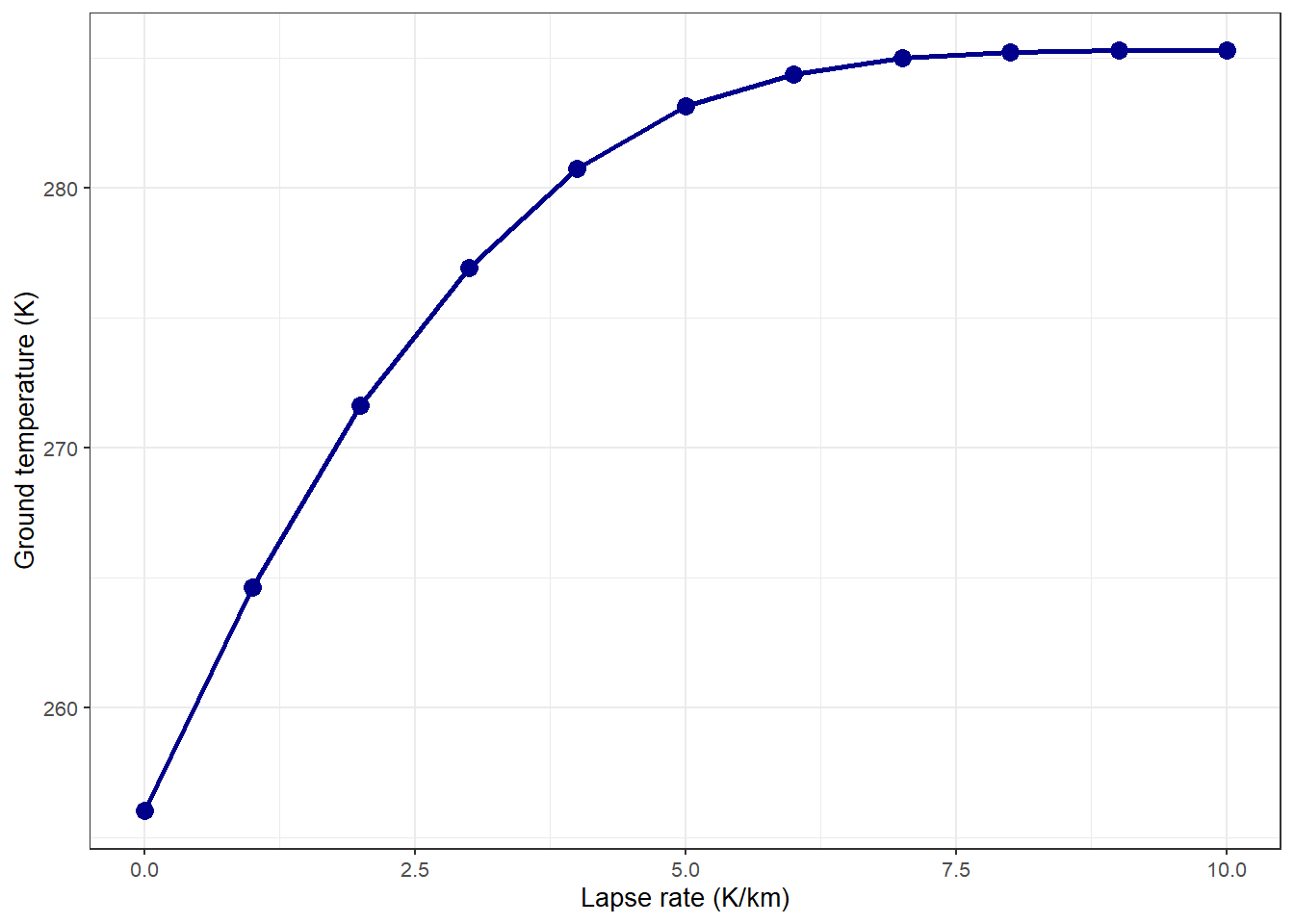
Figure 1: Equilibrium surface temperature versus lapse rate.

Explanation:

You don’t need to have as much detail in your answer as I put in this explanation.

The reason this is happening is that the closer the basic environmental lapse rate gets to the dry adiabatic lapse rate, the less stable the atmosphere is and the easier it is for solar heating of the surface to set off convection that redistributes heat (basically bringing heat from the surface to the upper troposphere).

When the environmental lapse rate (ELR) is less than the moist adiabatic lapse rate, the surface temperature is close to \(T_{\text{surface}} = T_{\text{skin}} + h_{\text{skin}} \text{ELR}\), but when the ELR becomes greater than the moist adiabatic lapse rate, there is so much convection that it disrupts the simple picture I presented in class.

The picture I presented in class works well for an atmosphere like ours, which is marginally stable (i.e., the environmental lapse rate is roughly equal to the average moist adiabatic lapse rate). When the atmosphere is undergoing a large amount of constant convection, then heat flow behaves differently.

All of that convection transports lots of heat from the surface to the upper troposphere and brings lots of cold air down from the upper troposphere to the surface, which makes it hard for the surface to get warmer. This is why the ground temperature flattens out and stops changing very much after the lapse rate reaches about 6 K/km.

Exercise 2: Skin Altitude

Answer this question using the online MODTRAN IR radiation model at https://climatemodels.jgilligan.org/modtran/ or http://climatemodels.uchicago.edu/modtran/.

From the notes in the assignment:

The MODTRAN model ignores shortwave light and only considers longwave (infrared) light emitted by the earth’s surface and atmosphere. When you start it up, you pick a locality (for this exercise, use “Tropical Atmosphere” just as you did for the exercises in Chapter 4) and the model will initialize to conditions of radiative balance at that locality (for the tropical atmosphere, this is 298.52 W/m²). You can then adjust all sorts of parameters (the concentrations of different gases, the conditions of clouds or rain, and the temperature of the ground), and the model will calculate the new upward longwave heat flux at the altitude you specify. You want to make a note of the upward IR heat flux for the default conditions before you start changing things, and then when you change parameters, such as the amount of CO₂ in the atmosphere, you can adjust the ground temperature until the upward IR heat flux returns to its initial value.

and

For exercise 2, use the MODTRAN model. Choose “Tropical Atmosphere” for Location and keep the altitude at its default value of 70 km. How would you calculate the skin altitude from this model?

Now, back to the exercise from the textbook:

1. Run the model in some configuration without clouds and with present-day \(p\ce{CO2}\). Compute \(\sigma T^4\) using the ground temperature to estimate the heat flux that you would get if there were no atmosphere. The value of \(\sigma\) is \(5.67 \times 10^{-8}~\mathrm{W}/(\mathrm{m}^2 \mathrm{K}^4)\). Is the model heat flux at the top of the atmosphere higher or lower than the heat flux you calculated at the ground?

From the notes in the assignment:

There’s a typo in exercise 2(a): The Stefan-Boltzmann constant should be \(\sigma = 5.67 \times 10^{-8} \mathrm{W/m^2 K^4}\) (\(10^{-8}\), not \(10^8\))